森林分野における衛星データ利用事例
この章で学習すること
本章では、茨城県日立市を対象に、衛星データからNDVIを算出し、森林の状態変化を可視化する方法を学びます。
numpyを用いた画像解析処理演算rasterioを用いたカラー合成画像の作成とマスク処理rasterioを用いたNDVIの計算matplotlibを用いたグラフ作成
背景
持続可能な開発目標(SDGs)の目標14は「海の豊かさを守ろう」ですが、目標15では「陸の豊かさも守ろう」が定められています。陸域生態系の保護や土地劣化の阻止などと並び、森林は重要な要素であり、例えば以下のようなターゲットが含まれています(数字はターゲット番号)。
- 森林を含む陸域生態系の保全・回復・持続可能な利用(15.1)
- 持続可能な森林経営、森林減少阻止、劣化した森林の回復(15.2)
- 持続可能な森林経営のための資金の調達と開発途上国への資源の動員(15.b)
適切な森林経営のためには現状の把握と監視が必要であり、大規模な森林を把握・監視するためには衛星が有効な手段です。
光学衛星で森林を監視する手段として、今回は植生指標に着目します。森林を含む全ての植物は近赤外線を反射し、可視光線のうち赤色の波長を吸収する特性があります。この近赤外と赤色の分光反射率を組み合わせることで植生指標を算出し、森林など植生の状態把握をすることが可能です。
この章では、一般的に用いられている植生指標としてNDVI(Normalized Difference Vegetation Index)を衛星データから計算し、それを時系列に可視化します。植生指数は、森林から他の土地被覆に変化した場合だけでなく季節によっても変化します。そのため、時系列で森林を解析するためには、まず、対象となる地域における季節と植生指標との関係を確認することがとても重要です。ここでは、森林の植生指標の季節変化を可視化する方法を学んでいきます。
準備
# google driveをマウント
# Tellusの開発環境やローカル環境を使用する想定であれば、このセルは削除可です。
from google.colab import drive
drive = drive.mount('/content/drive')
必要なライブラリのインストール
!pip install collection
!pip install rasterio
!apt install gdal-bin python-gdal python3-gdal
!apt install python3-rtree
!pip install git+git://github.com/geopandas/geopandas.git
!pip install descartes
!pip install shapely
!pip install six
!pip install pyproj
!pip install pandas
!pip install geopandas

print("done")
ライブラリのインポート
「基礎編」でご紹介したGDALライブラリは、地理空間データを扱う上で基礎となる重要なライブラリですが、GISの概念に慣れていないと理解しにくいパラメータがたくさん登場するため、衛星データを触り始めたばかりの頃は複雑に感じることもあるかと思います。
この教材では、地理空間データの処理がより便利になるPythonのライブラリをいくつかご紹介します。
-
numpyは、数値計算を効率的に行うための拡張モジュールです。基本的な計算はpythonだけでも出来ますが、numpyを使うとその計算が高速になったり、より楽になったりします。多次元配列を必要とする処理において、特にその機能を発揮するライブラリです。 -
rasterioは、オンラインマッププロバイダーのMapboxが中心となって開発しているOSSのライブラリで、衛星データでは最も一般的なGeoTiffフォーマットのデータを扱う際に、シンプルな書き方ができるのが特徴のライブラリです。
-
matplotlibは、Pythonでグラフや図を描画、作成するための包括的なライブラリです。折れ線グラフやヒストグラムといった2次元グラフだけなく3次元のグラフも描画することが可能です。
#必要ライブラリのインポート
import os
import numpy as np
import geopandas as gpd
import pandas as pd
import matplotlib.pyplot as plt
import rasterio as rio
import rasterio.mask
import fiona
import folium
import zipfile
import glob

from mpl_toolkits.axes_grid1 import make_axes_locatable
from shapely.geometry import MultiPolygon, Polygon
from rasterio import plot
from rasterio.plot import show
from rasterio.plot import plotting_extent
from rasterio.mask import mask
from PIL import Image
from osgeo import gdal

print("done")
衛星データの取得
この章では、ヨーロッパ宇宙機関(ESA)が運用するSentinel-2衛星が取得するデータを使用します。ESAのオープンデータポリシーに基づき、誰でも無償で観測データを利用することが可能です。
Sentinel-2について
Sentinel-2は陸域観測を主目的とした光学衛星であり、可視光、近赤外を含む12種類の異なる波長帯(バンド)で観測を行っています。
光学衛星は雲があると地表を観測できませんが、Sentinel-2は同じ設計の衛星2機を運用することで、5日に1回の観測を可能とし、晴天時のデータを入手できる可能性を高めています。
以下の2種類のプロダクトが提供されています。今回はLevel-1Cのプロダクトを使用します。
- Level-1C: 建物の倒れこみ等、幾何学的な歪みを補正したオルソ補正済みプロダクト
- Level-2A: 1Cの補正に加え、大気の吸収・散乱の影響を軽減し、地表面の反射率に変換した大気補正済みプロダクト
衛星の緒言についてはリモート・センシング技術センターのサイトを参照してください。
データの検索とダウンロード
データを取得するに際し、ESAのサイトCopernicus Open Access Hubでユーザ登録を行いましょう。ユーザー登録の詳細はこちらを参照してください。
Copernicus Open Access Hubの検索画面(図1)で、地図上で対象領域を指定した上で、以下の条件を入力して検索しましょう。今回は茨城県の日立市を対象としてデータを検索します。
- 「Sensing period」(観測期間)に下記の期間を入力。
2017年 → 2017年1月1日から12月31日
2018年 → 2018年1月1日から12月31
- 「Mission: Sentinel-2」のチェックボックスにチェック。
- 「Product type」はプルダウンで「S2MSI1C」を選択。
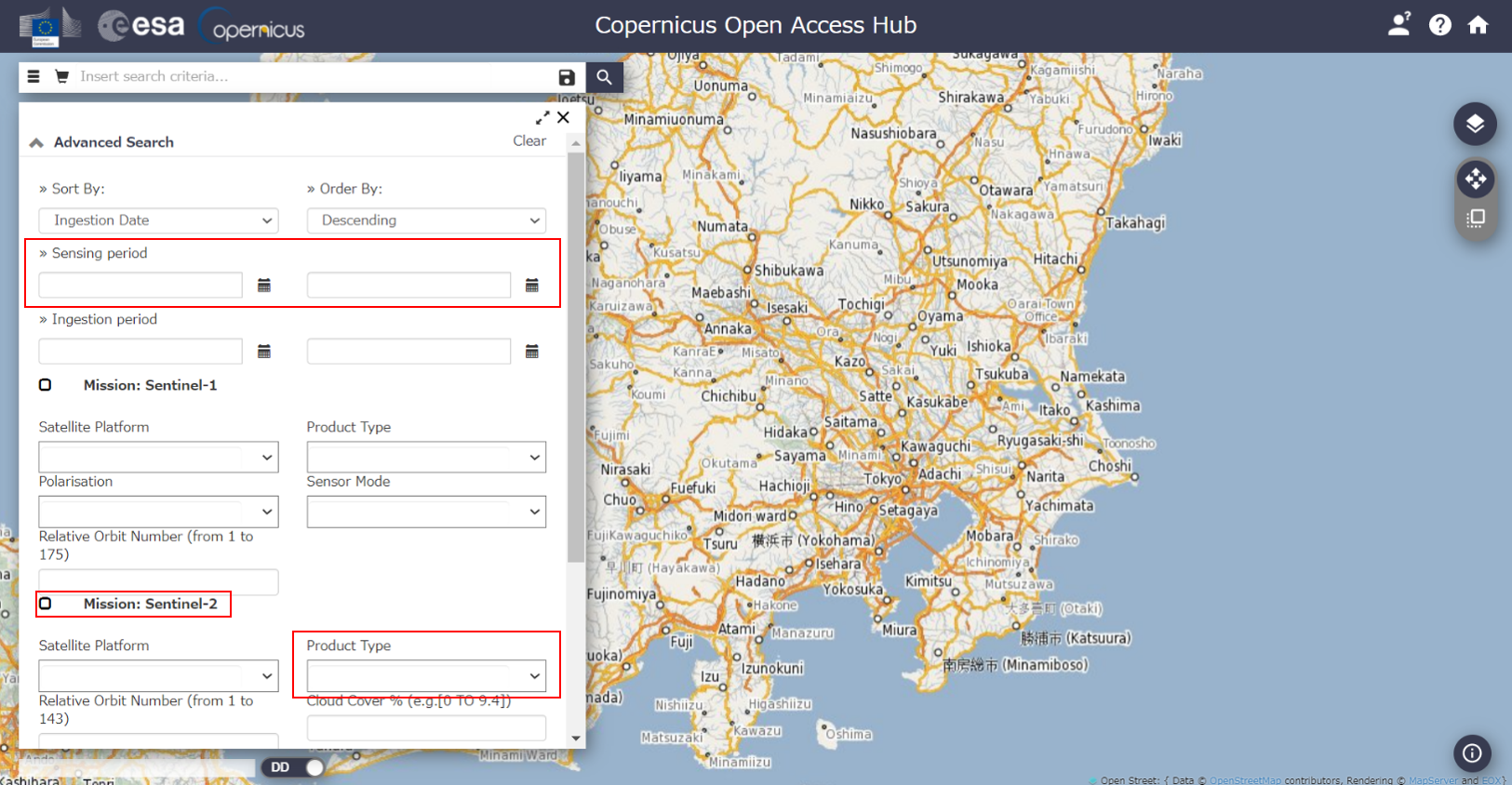
検索したデータはサムネイル画像で雲の様子などが確認できるので、雲が無い良好なデータを見つけましょう。
今回は、2017年5月から2018年12月の7シーンのデータを使って年間の森林状態の変化を確認し、2017年および2018年の5月のデータを使って経年変化を確認します。
使用するデータ(全7シーン)の日付は以下の通りです。
- 2017-05-08
- 2017-10-27
- 2017-12-26
- 2018-04-20
- 2018-05-20
- 2018-10-02
- 2018-12-19
Coperniqus Open Access Hubからデータをダウンロードすると、zip形式で圧縮されているので展開します。
# Tellusの開発環境やローカル環境を使用する想定であれば、適切なパスに書き換えてください。

a = glob.glob('/content/drive/MyDrive/s2/*.zip')

ziplis = []

for f in a:
  print(f[26:86])
  ziplis.append(f[26:86])

for file_title in ziplis:
  print("start unzip:"+ file_title)
  file_name = file_title +".zip"
  file_dir = "/content/drive/MyDrive/s2/"
  file_pass = os.path.join(file_dir + file_name)
  print(file_pass)
  with zipfile.ZipFile(file_pass) as zf:
    zf.extractall()
  print("done")
解析結果を格納するための作業用ディレクトリを以下のように準備します。このディレクトリには、workディレクトリの下にTIF、NDVIおよびNDVIにマスク処理をしたデータを保存するためのディレクトリを作成します。
#作業用ディレクトリ(フォルダ)の作成

os.mkdir("work")

path = '/content/'
work_path = '/content/work'

RGB_dir = '/content/work/RGB_TIF'
os.mkdir(RGB_dir)

NDVI_dir = '/content/work/NDVI'
os.mkdir(NDVI_dir)

NDVI_mask_dir = '/content/work/NDVI_mask'
os.mkdir(NDVI_mask_dir)
コラム:API経由のLTAデータ取得
Sentinel-2のデータはAPI経由でも取得することが可能で、宙畑の記事で取得方法が紹介されています。
ただし、2019年8月以前に観測されたSentinel-2のLevel 2Aデータは全てLTA(Long Term Archives)に保管されており、それらデータをAPIで取得したい場合はESAにリクエストを送る必要があります。リクエストが承認されると、24時間以内にプロダクトがダウンロード可能となり、その時点から3日間利用可能となります。
2019年9月以降に観測されたデータであれば、常時取得が可能なのでリクエストを送らずにAPIで取得できます。
今回はAPIを使わずにデータを取得しましたが、APIでのデータ取得もぜひお試しください。
※2020年12月現在、複数のLTAデータを同時にリクエストすることができない状態となっています。リクエストは30分ごとに1回しか送信できないため、多くのシーンを取得したい場合は非常に時間がかかります。
カラー合成画像の作成
今回の解析では茨城県日立市の森林を対象としますので、それ以外の領域は不要です。対象領域のみを解析するため、国土地理院が公開しているポリゴンデータ(Shapefile)を使って不要な領域をマスク(隠す)します。
#ダウンロードしたデータを解凍して、ディレクトリを指定
shape_path = "/content/drive/MyDrive/N03-20200101_08_GML/"

# 茨城県のshpの読み込み
in_shape = gpd.read_file(os.path.join(shape_path + "N03-20_08_200101.shp"),encoding="shift-jis")

# 日立市でソート
shape_srt = in_shape[in_shape["N03_004"].isin(["日立市"])]
shape_srt = shape_srt.drop(columns=["N03_002","N03_003"])

#画像に合わせて投影変換
out_file = os.path.join(shape_path + "re_N03-20_08_200101.shp")
re_shape = shape_srt.to_crs({"init": "epsg:32654"})

#出力
re_shape.to_file(driver="ESRI Shapefile",filename=out_file)
print("done")

#GeoDataFrameを描画
f,ax = plt.subplots(1, figsize=(6,6))
ax = re_shape.plot(axes=ax)
plt.show

カラー合成とマスク処理
Sentinel-2は異なる12の波長帯(バンド)で観測していると説明しましたが、ダウンロードしたデータはバンド毎にjpeg2の形式で格納されています。
まずは、基礎分野で学習した「トゥルーカラー(True Color)」の組み合わせでカラー合成し、日立市以外の領域をマスクしてみましょう。
ここではrasterioで、バンド2(青)・バンド3(緑)・バンド4(赤)を組み合わせて合成し、ポリゴンデータを使って日立市以外をマスクします。
for file_title in ziplis:
  print("Start make RGB TIF image " +'<'+ file_title +'>')

  path_A = str(file_title) + '.SAFE/GRANULE/'
  f1 = os.listdir(path_A)
  path_B = str(file_title) + '.SAFE/GRANULE/' + str(f1[0])
  f2 = os.listdir(path_B)
  path_C = str(file_title) + '.SAFE/GRANULE/' + str(f1[0]) + '/IMG_DATA/'
  f3 = os.listdir(path_C)

  b2 = rio.open(str(file_title) + '.SAFE/GRANULE/' + str(f1[0]) +'/IMG_DATA/' +str(f3[0][0:23] +'B02.jp2'))
  b3 = rio.open(str(file_title) + '.SAFE/GRANULE/' + str(f1[0]) +'/IMG_DATA/' +str(f3[0][0:23] +'B03.jp2'))
  b4 = rio.open(str(file_title) + '.SAFE/GRANULE/' + str(f1[0]) +'/IMG_DATA/' +str(f3[0][0:23] +'B04.jp2'))

  RGB_path = os.path.join(RGB_dir,'sentinel-2_'+str(f3[0][7:15])+'_RGB.tif')


  RGB_colar = rio.open(RGB_path,'w',driver='Gtiff',
                       width=b4.width, height=b4.height,
                       count=3,
                       crs=b4.crs,
                       transform=b4.transform,
                       dtype=rasterio.uint16
                       )
  RGB_colar.write(b2.read(1),3)
  RGB_colar.write(b3.read(1),2)
  RGB_colar.write(b4.read(1),1)
  RGB_colar.close()

  print("---masking---")

  with fiona.open(out_file, "r") as mask:
    masks = [feature["geometry"] for feature in mask]

  with rasterio.open(RGB_path) as src:
    out_image, out_transform = rasterio.mask.mask(src, masks, crop=True)
    out_meta = src.meta

  out_meta.update({"driver": "GTiff",
                 "height": out_image.shape[1],
                 "width": out_image.shape[2],
                 "transform": out_transform})

  with rasterio.open(RGB_path, "w", **out_meta) as dest:
    dest.write(out_image)

  #画像表示のため8bit形式で書き出し。
  scale = '-scale 0 255 0 15'
  options_list = ['-ot Byte','-of Gtiff',scale]
  options_string = " ".join(options_list)

  gdal.Translate(os.path.join(RGB_dir + "/" + 'sentinel-2_'+str(f3[0][7:15])+'.tif'),os.path.join(RGB_dir + "/" + 'sentinel-2_'+str(f3[0][7:15])+'_RGB.tif'),options = options_string)

  print("Done")
plt.figure(figsize=(18,9))

RGB_2018_spring = rio.open(RGB_dir+'/sentinel-2_20180420.tif')
RGB_2018_summer = rio.open(RGB_dir+'/sentinel-2_20180520.tif')
RGB_2018_autumn = rio.open(RGB_dir+'/sentinel-2_20181002.tif')
RGB_2018_winter = rio.open(RGB_dir+'/sentinel-2_20181219.tif')

ax1 = plt.subplot(1,4,1)
ax1.set_title("RGB_2018_spring")
ax2 = plt.subplot(1,4,2)
ax2.set_title("RGB_2018_summer")
ax3 = plt.subplot(1,4,3)
ax3.set_title("RGB_2018_autumn")
ax4 = plt.subplot(1,4,4)
ax4.set_title("RGB_2018_winter")

show(RGB_2018_spring.read([1,2,3]),ax=ax1)
show(RGB_2018_summer.read([1,2,3]),ax=ax2)
show(RGB_2018_autumn.read([1,2,3]),ax=ax3)
show(RGB_2018_winter.read([1,2,3]),ax=ax4)

2018年の4シーン(4月、5月、10月、12月)のカラー合成画像です。見た目にはほとんど違いは分かりません。
森林の状態変化の可視化
#森林マップポリゴン

#ダウンロードしたデータを解凍して、ディレクトリを指定
mori_shape_path = "/content/drive/MyDrive/A13-15_08_GML/"

# 森林マップポリゴンの読込(森林域のポリゴンは下2桁が07)
mori_shape = gpd.read_file(os.path.join(mori_shape_path + "a001080020160207.shp"),encoding="shift-jis")

#画像に合わせて投影変換
out_file_mori = os.path.join(mori_shape_path + "re_a001080020160207.shp")
re_mori_shape = mori_shape.to_crs({"init": "epsg:32654"})

#出力
re_mori_shape.to_file(driver="ESRI Shapefile",filename=out_file_mori)
print("done")

#GeoDataFrameを描画
f,ax = plt.subplots(1, figsize=(6,6))
ax = re_mori_shape.plot(axes=ax)
plt.show

茨城県の森林地域のポリゴンです。青い部分が森林になります。
正規化植生指数(NDVI)
植生の活性度を見るためには、正規化植生指数(Normalized Difference Vegetation Index: NDVI)という指数を使うことが有効です。NDVIは、近赤外線(NIR)と赤色(Red)の波長帯のデータを使って、以下の計算式で求めることができます。
$ NDVI=(NIR-Red)/(NIR+Red)$
</br>
Sentinel-2の場合、バンド4で赤色、バンド8で近赤外線を使っているので、以下の式でNDVIを算出します。
$NDVI=(Band 8-Band 4)/(Band 8+Band 4)$
</br>
なお、NDVIについては宙畑の記事でも紹介されているので参考にしてください。
日立市におけるNDVIを計算します。 Sentinel-2で雲の無いデータを取得できた4時期(4月、5月、10月、12月)全てでNDVIを計算します。
NDVI_dir = '/content/work/NDVI'

for file_title in ziplis:
  print("Start make NDVI " +'<'+ file_title +'>')

  path_A = str(file_title) + '.SAFE/GRANULE/'
  f1 = os.listdir(path_A)

  path_B = str(file_title) + '.SAFE/GRANULE/' + str(f1[0])
  f2 = os.listdir(path_B)

  path_C = str(file_title) + '.SAFE/GRANULE/' + str(f1[0]) + '/IMG_DATA/'
  f3 = os.listdir(path_C)

  b4 = rio.open(str(file_title) + '.SAFE/GRANULE/' + str(f1[0]) +'/IMG_DATA/' +str(f3[0][0:23] +'B04.jp2'))
  b8 = rio.open(str(file_title) + '.SAFE/GRANULE/' + str(f1[0]) +'/IMG_DATA/' +str(f3[0][0:23] +'B08.jp2'))

  red = b4.read()
  nir = b8.read()

  ndvi = np.where(((red != 0) & (nir != 0)),(nir.astype(float)-red.astype(float))/(nir.astype(float)+red.astype(float)), 0)

  out_meta = b4.meta
  out_meta.update(driver='GTiff')
  out_meta.update(dtype=rasterio.float32)

  NDVI_path = os.path.join(NDVI_dir,'sentinel-2_'+str(f3[0][7:15])+ '_ndvi.tif')

  with rio.open(NDVI_path, 'w', **out_meta) as dst:
    dst.write(ndvi.astype(rasterio.float32))

  print("---masking---")

  with fiona.open(out_file, "r") as mask:
    masks = [feature["geometry"] for feature in mask]

  with rio.open(NDVI_path) as src2:
    out_image_ndvi, out_transform = rasterio.mask.mask(src2, masks, crop=True)
    out_meta = src2.meta

  out_meta.update({"driver": "GTiff",
                 "height": out_image.shape[1],
                 "width": out_image.shape[2],
                 "transform": out_transform})

  with rasterio.open(NDVI_path, "w", **out_meta) as dst2:
    dst2.write(out_image_ndvi)

  print("Done")
次に画像を表示します。
fig,(ax1,ax2,ax3,ax4)=plt.subplots(1,4, figsize=(18,9))
plt.subplots_adjust(wspace=0.4)

NDVI_2018_spring = rio.open(NDVI_dir+'/sentinel-2_20180420_ndvi.tif')
NDVI_2018_summer = rio.open(NDVI_dir+'/sentinel-2_20180520_ndvi.tif')
NDVI_2018_autumn = rio.open(NDVI_dir+'/sentinel-2_20181002_ndvi.tif')
NDVI_2018_winter = rio.open(NDVI_dir+'/sentinel-2_20181219_ndvi.tif')

NDVI_2018_spring = NDVI_2018_spring.read(1)
NDVI_2018_summer = NDVI_2018_summer.read(1)
NDVI_2018_autumn = NDVI_2018_autumn.read(1)
NDVI_2018_winter = NDVI_2018_winter.read(1)

ndvi1=ax1.imshow(NDVI_2018_spring, cmap='RdYlGn')
ax1.set_title("NDVI_2018_spring")
ndvi1.set_clim(vmin=-1, vmax=1)
divider = make_axes_locatable(ax1)
ax_cb = divider.new_horizontal(size="5%", pad=0.1)
fig.add_axes(ax_cb)
plt.colorbar(ndvi1, cax=ax_cb)

ndvi2=ax2.imshow(NDVI_2018_summer, cmap='RdYlGn')
ax2.set_title("NDVI_2018_summer")
ndvi2.set_clim(vmin=-1, vmax=1)
divider = make_axes_locatable(ax2)
ax_cb = divider.new_horizontal(size="5%", pad=0.1)
fig.add_axes(ax_cb)
plt.colorbar(ndvi2, cax=ax_cb)

ndvi3=ax3.imshow(NDVI_2018_autumn, cmap='RdYlGn')
ax3.set_title("NDVI_2018_autumn")
ndvi3.set_clim(vmin=-1, vmax=1)
divider = make_axes_locatable(ax3)
ax_cb = divider.new_horizontal(size="5%", pad=0.1)
fig.add_axes(ax_cb)
plt.colorbar(ndvi3, cax=ax_cb)

ndvi4=ax4.imshow(NDVI_2018_winter, cmap='RdYlGn')
ax4.set_title("NDVI_2018_winter")
ndvi4.set_clim(vmin=-1, vmax=1)
divider = make_axes_locatable(ax4)
ax_cb = divider.new_horizontal(size="5%", pad=0.05)
fig.add_axes(ax_cb)
plt.colorbar(ndvi4, cax=ax_cb)

実際に作成したNDVIの画像を表示しました。画像左から順に、4月⇒5月⇒10月⇒12月のNDVI画像となっています。
これらの画像では画像同士の違いを比較しやすくするために、NDVIの範囲を-1から1に揃えています。
また、NDVIの値が1に近い(緑色が強い)ほど植物の活性が高いことを示しており、-1に近い(赤が強い)ほど植生が少ないことを示しています。
先ほどのカラー合成画像と見比べると、森林と思われる地域のNDVIはほとんど緑色になっていることがわかります。
森林地域のNDVIの計算
今回は森林を対象としているので、ポリゴンデータを使って不要な領域をマスク処理し、日立市の森林地域のみNDVIを計算してみましょう。
NDVI_dir = '/content/work/NDVI'

for file_title in ziplis:
  print("Start masking NDVI " +'<'+ file_title +'>')
  path_A = str(file_title) + '.SAFE/GRANULE/'
  f1 = os.listdir(path_A)

  path_B = str(file_title) + '.SAFE/GRANULE/' + str(f1[0])
  f2 = os.listdir(path_B)

  path_C = str(file_title) + '.SAFE/GRANULE/' + str(f1[0]) + '/IMG_DATA/'
  f3 = os.listdir(path_C)

  NDVI_path = os.path.join(NDVI_dir,'sentinel-2_'+str(f3[0][7:15])+ '_ndvi.tif')

  with fiona.open(out_file_mori, "r") as mask_mori:
    masks_mori = [feature["geometry"] for feature in mask_mori]
  with rio.open(NDVI_path) as src3:
    out_image_ndvi, out_transform = rasterio.mask.mask(src3, masks_mori, crop=True)
    out_meta = src3.meta
  out_meta.update({"driver": "GTiff","height": out_image.shape[1],"width": out_image.shape[2],"transform": out_transform})

  NDVI_mask_path = os.path.join(NDVI_mask_dir,'sentinel-2_'+str(f3[0][7:15])+ '_ndvi_mask.tif')

  with rasterio.open(NDVI_mask_path, "w", **out_meta) as dest3:
    dest3.write(out_image_ndvi)
  print("done")
次に画像を表示します。
fig,(ax1,ax2,ax3,ax4)=plt.subplots(1,4, figsize=(18,9))
plt.subplots_adjust(wspace=0.4)

NDVI_2018_spring = rio.open(NDVI_mask_dir+'/sentinel-2_20180420_ndvi_mask.tif')
NDVI_2018_summer = rio.open(NDVI_mask_dir+'/sentinel-2_20180520_ndvi_mask.tif')
NDVI_2018_autumn = rio.open(NDVI_mask_dir+'/sentinel-2_20181002_ndvi_mask.tif')
NDVI_2018_winter = rio.open(NDVI_mask_dir+'/sentinel-2_20181219_ndvi_mask.tif')

NDVI_2018_spring = NDVI_2018_spring.read(1)
NDVI_2018_summer = NDVI_2018_summer.read(1)
NDVI_2018_autumn = NDVI_2018_autumn.read(1)
NDVI_2018_winter = NDVI_2018_winter.read(1)

ndvi1=ax1.imshow(NDVI_2018_spring, cmap='RdYlGn')
ax1.set_title("NDVI_2018_spring")
ndvi1.set_clim(vmin=-1, vmax=1)
divider = make_axes_locatable(ax1)
ax_cb = divider.new_horizontal(size="5%", pad=0.1)
fig.add_axes(ax_cb)
plt.colorbar(ndvi1, cax=ax_cb)

ndvi2=ax2.imshow(NDVI_2018_summer, cmap='RdYlGn')
ax2.set_title("NDVI_2018_summer")
ndvi2.set_clim(vmin=-1, vmax=1)
divider = make_axes_locatable(ax2)
ax_cb = divider.new_horizontal(size="5%", pad=0.1)
fig.add_axes(ax_cb)
plt.colorbar(ndvi2, cax=ax_cb)

ndvi3=ax3.imshow(NDVI_2018_autumn, cmap='RdYlGn')
ax3.set_title("NDVI_2018_autumn")
ndvi3.set_clim(vmin=-1, vmax=1)
divider = make_axes_locatable(ax3)
ax_cb = divider.new_horizontal(size="5%", pad=0.1)
fig.add_axes(ax_cb)
plt.colorbar(ndvi3, cax=ax_cb)

ndvi4=ax4.imshow(NDVI_2018_winter, cmap='RdYlGn')
ax4.set_title("NDVI_2018_winter")
ndvi4.set_clim(vmin=-1, vmax=1)
divider = make_axes_locatable(ax4)
ax_cb = divider.new_horizontal(size="5%", pad=0.05)
fig.add_axes(ax_cb)
plt.colorbar(ndvi4, cax=ax_cb)

森林地域以外をマスクしたNDVIの画像を表示しました。画像左から順に、4月⇒5月⇒10月⇒12月のNDVI画像となっています。
先ほどと同様に、画像同士の違いを比較しやすくするために、NDVIの範囲を-1から1に揃えています。
マスク処理をすることにより、都市部など森林以外の地域が除外することができました。
森林状態変化のグラフ表示
作成したNDVI画像を用いて森林地域の変化を推定し、可視化します。 本章ではポリゴンによって抜き出した範囲を森林地域として、範囲内のNDVI変化をみることで、森林の状態変化を推定します。
はじめに森林地域のNDVI値を集計して平均値、最大値、最小値を算出します。
#NDVI値の集計
NDVI_list = os.listdir(NDVI_mask_dir)

NDVI_files = []
ind = []
col = []
NDVI_max=[]
NDVI_min=[]
value_ave=[]

#for seane in sorted(NDVI_list):
#  if "2018" in seane:
#    NDVI_files.append(seane)

for seane in sorted(NDVI_list):
   NDVI_files.append(seane)

for seane in sorted(NDVI_files):
  print("Start " +'<'+ seane +'>')
  NDVI_image = rio.open(NDVI_mask_dir +"/"+ seane)
  NDVI_image_2 = NDVI_image.read()
  ind.append('NDVI_forest' + '_' + str(seane[11:19]))
  col.append('NDVI_' + str(seane[15:22]))
  NDVI_max.append(np.max(NDVI_image_2))
  NDVI_min.append(np.min(NDVI_image_2))
  NDVI_value = NDVI_image_2[np.nonzero(NDVI_image_2)].mean()
  value_ave.append(NDVI_value)
  print("done")
計算した結果を用いて、各時期のNDVI平均値を正規化します。
7時期の中でNDVIの値が最も高いと考えられる5月のNDVI平均値を全体の最大値、最も数値の低いと考えられる12月のNDVI値を全体の最小値とします。
NDVI_normalized = []

for va in value_ave:
  nor = ((va - NDVI_min[3])/(NDVI_max[1] - NDVI_min[3]))
  NDVI_normalized.append(nor)
print("done")
正規化した値の中で、植生が最も活性化する夏季(本章では5月)の正規化NDVI平均値を基準に日立市における森林面積に対し、各季節と夏季の比率を積算することで、季節変化による森林の状態の変移を推定します。
日立市における森林面積は森林域をマスクする際に使用した国土数値情報および農林水産省のデータを参照し12,065haとしました。
また、参照した国土数値情報および農林水産省のデータはいずれも2020年12月時点で最新版のものを使用しています。
forest_area = 12065

forest = []

for seasonal_data in NDVI_normalized:
  est_fore = forest_area * (seasonal_data/NDVI_normalized[1])
  forest.append(est_fore)

print("done")
fig,ax1 = plt.subplots(1,1,figsize=(20,8))
ax1.plot(ind,forest,color="green")
ax1.set_xlabel("date",fontsize=20)
ax1.set_ylabel("Forest area estimated from NDVI [ha]",fontsize=20)
ax1.grid(True)
plt.title("Forest area detection at hitachi city",fontsize=20)
fig.show()

日立市の森林は2017年の5月から12月にかけて減少し、4月から5月に向けて繁茂している森林の面積が増加しています。その後、2018年の5月から10月にかけて減少し、12月にはさらに落ち込んでいます。
樹木は主に常緑樹と落葉樹の2つに分類できますが、NDVIは葉の活性度と相関性があるため、12月の減少は落葉による影響と考えられます。このことから、日立市の森林は落葉樹が多いと考えられます。
5月のデータは2018年の方が数値が高いですが、2017年は5月8日、2018年は5月20日のデータです。仮に、2017年の5月下旬のデータが撮れていれば、2018年と同様の数値になったのではないかと考えられます。また、天候の違いによって生長の時期に差が生じている可能性もあります。
次に2017年と2018年の5月のNDVI画像を比較してみます。
fig,(ax1,ax2)=plt.subplots(1,2, figsize=(18,9))
plt.subplots_adjust(wspace=0.4)

NDVI_2017 = rio.open(NDVI_dir+'/sentinel-2_20170508_ndvi.tif')
NDVI_2018 = rio.open(NDVI_dir+'/sentinel-2_20180520_ndvi.tif')


NDVI_2017 = NDVI_2017.read(1)
NDVI_2018 = NDVI_2018.read(1)

ndvi1=ax1.imshow(NDVI_2017, cmap='RdYlGn')
ax1.set_title("NDVI_20170508")
ndvi1.set_clim(vmin=-1, vmax=1)
divider = make_axes_locatable(ax1)
ax_cb = divider.new_horizontal(size="5%", pad=0.1)
fig.add_axes(ax_cb)
plt.colorbar(ndvi1, cax=ax_cb)

ndvi2=ax2.imshow(NDVI_2018, cmap='RdYlGn')
ax2.set_title("NDVI_20180520")
ndvi2.set_clim(vmin=-1, vmax=1)
divider = make_axes_locatable(ax2)
ax_cb = divider.new_horizontal(size="5%", pad=0.1)
fig.add_axes(ax_cb)
plt.colorbar(ndvi2, cax=ax_cb)

また、画像の上側中央付近においてNDVIの数値が落ち込んでいる地点が見受けられます。
二時期のNDVIの差分を取り、切り出してみましょう。またカラー合成画像から同様の範囲を切り出して、NDVIの差分画像と比較してみましょう。
#範囲の指定
minX = 750
minY = 400
deltaX = 300
deltaY = 300

#NDVI差分の作成
NDVI_2017 = rio.open(NDVI_dir+'/sentinel-2_20170508_ndvi.tif')
NDVI_2018 = rio.open(NDVI_dir+'/sentinel-2_20180520_ndvi.tif')

ndvi_2017 = NDVI_2017.read()
ndvi_2018 = NDVI_2018.read()

ndvi_diff = np.where(((ndvi_2017 != 0) & (ndvi_2018 != 0)),(ndvi_2018.astype(float)-ndvi_2017.astype(float)), 0)

out_meta = NDVI_2017.meta
out_meta.update(driver='GTiff')
out_meta.update(dtype=rasterio.float32)

NDVI_diff_path = os.path.join(NDVI_dir,'sentinel-2_ndvi_diff.tif')

with rio.open(NDVI_diff_path, 'w', **out_meta) as dst:
  dst.write(ndvi_diff.astype(rasterio.float32))

path_ndvi_diff = "/content/work/NDVI/sentinel-2_ndvi_diff.tif"

#NDVI差分画像の切り出し
print("Start cliping images " +'<'+ str(path_ndvi_diff) +'>')
maskdata_path = os.path.join(NDVI_dir + "/" + "ndvi_diff_clip.tif")
ds=gdal.Translate(maskdata_path, path_ndvi_diff, srcWin=[minX,minY,deltaX,deltaY])

#RGB画像の指定
path_2017 = "/content/work/RGB_TIF/sentinel-2_20170508.tif"
path_2018 = "/content/work/RGB_TIF/sentinel-2_20180520.tif"

ln = [path_2017,path_2018]

#切り出し
for n in ln:
  print("Start cliping images " +'<'+ n +'>')
  maskdata_path = os.path.join(RGB_dir + "/" + "clip_" + str(n[33:37]) + ".tif")
  ds=gdal.Translate(maskdata_path, n, srcWin=[minX,minY,deltaX,deltaY])
  ds=None
切り出した画像を表示します。
fig,(ax1,ax2,ax3) = plt.subplots(1,3,figsize=(18,18))

#画像の読み込み
cut_img2017=rio.open("/content/work/RGB_TIF/clip_2017.tif")
cut_img2018=rio.open("/content/work/RGB_TIF/clip_2018.tif")
cut_imgNDVI=rio.open("/content/work/NDVI/ndvi_diff_clip.tif")

ax1 = plt.subplot(1,3,1)
ax1.set_title("2017")
ax2 = plt.subplot(1,3,2)
ax2.set_title("2018")
ax3 = plt.subplot(1,3,3)
ax3.set_title("NDVI difference 2017 and 2018")

show(cut_img2017.read([1,2,3]),ax=ax1)
show(cut_img2018.read([1,2,3]),ax=ax2)

img_n = ax3.imshow(cut_imgNDVI.read(1), cmap=plt.cm.bwr)
img_n.set_clim(vmin=-1, vmax=1)
divider = make_axes_locatable(ax3)
cax = divider.append_axes("right",size="5%", pad=0.3)
cbar = plt.colorbar(img_n, cax=cax,ticks=[-1, 0, 1])

上の図は左から、2017年のカラー合成画像、2018年のカラー合成画像、2017年と2018年のNDVIの差分画像となっています。NDVI差分画像の範囲は-1から1をとっており、差分の値が1に近い(赤色が強い)ほど植物が増えていることを示しており、-1に近い(青色が強い)ほど植生が減少していることを示しています。
差分画像とカラー合成画像を見比べてみると、青色が強調されている地域では、森林と思われる地域が裸地に変化しているようです。 赤色が強調されている地域は、もともと裸地であった地域に植生が繁茂しているようです。これは落葉樹の展葉等に伴い、一時的に変化として表れていることが考えられます。 そのため、経年変化で比較する際にも、取得する衛星の観測時期を考慮する必要があるといえます。
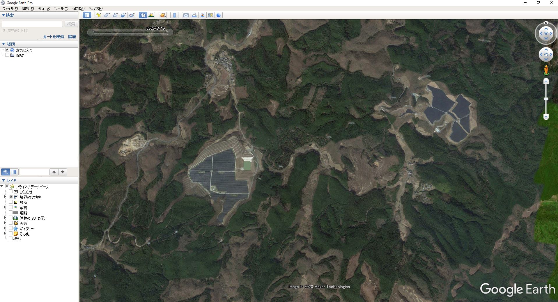
青色が強調されている地域の様子をGoogle Earthで見てみると、2020年3月時点でソーラーパネルによる発電施設が建設されていることがわかりました。
以上のことから、同じ年の複数時期の衛星データを比較することによって森林の状態変化を、別の年のデータを比較することで森林の増加や減少を確認することができました。NDVIの差分画像を使えば、広い範囲でも森林の伐採箇所を見つけやすくなります。
森林のNDVIは樹種によって季節で変化するため、衛星で森林の減少を監視するためには、適切な時期の衛星データを使うことが重要です。
まとめ
この章では、「Sentinel-2」と「国土数値情報」を使い、森林の時系列変化解析を通して、Pythonを用いた解析様々なライブラリの使い方ついて学習しました。 Sentinel-2衛星データは無料で入手できるので、ご自身の興味のある場所について、変化の解析をしてみてはいかがでしょうか。